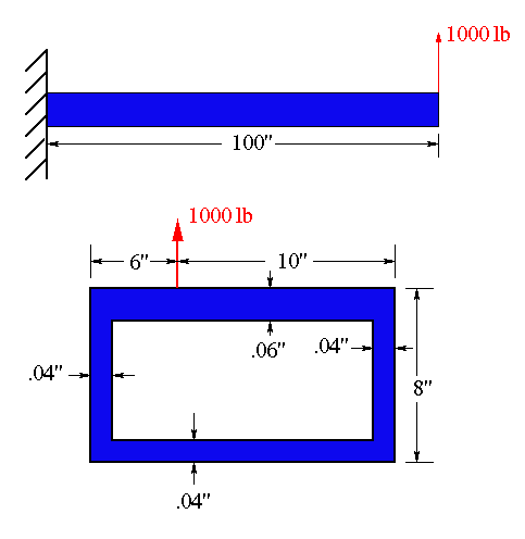
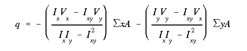
(a)
Due to vertical symmetry of the cross section, the shear center will lie on the centroidal y axis, hence ex = 0 in this case. However, with no symmetry about the horizontal centroidal axis, the value of ey is unknown.
Here is how we calculate the vertical coordinate of the shear center:
We consider the root section and apply a fictitious horizontal shear force Vx through the shear center. Note that the applied vertical load must be removed for this analysis. In this part we demonstrate the solution procedure described in case 1.
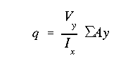
With no vertical force and no product of inertia, the general shear flow equation reduces to
Because of vertical cross-sectional symmetry and symmetric loading, the neutral axis will pass through the centroid as shown below.
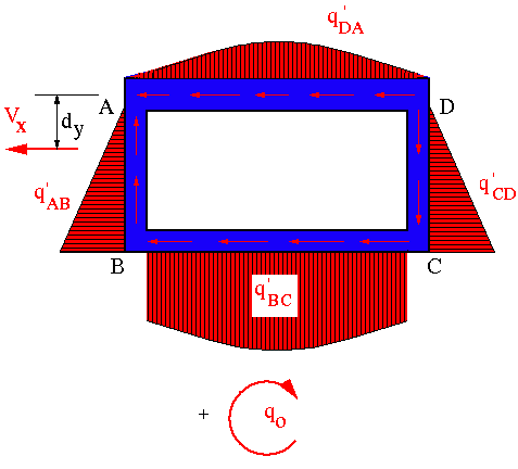
In order to use the general shear flow equation, we assume q = 0 at an arbitrary point. This assumption models the cross section as an "open" section. The resulting shear flow distribution is designated by q' to indicate that it only represents a preliminary and not the final shear flow distribution. We decided to assume q' = 0 at the upper left corner. We start from that point and go around the section and determine the preliminary shear flow distribution.
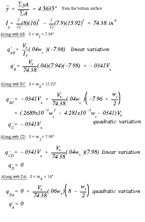
The resulting preliminary shear flow distribution due to Vx is shown below.
Since Vx passes through the shear center, the section will not twist. Using the angle of twist equation from chapter I and setting it to zero we obtain the constant shear flow q0 required to keep the section from twisting.
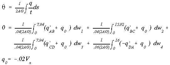
The negative sign on the shear flow q0 implies that its direction is opposite to that assumed in the figure above. The constant shear flow q0 is added to the preliminary shear flow system found previously to determine the final shear flow distribution (not shown here) due to Vx.
The direction of positive shear flow is arbitrary, in this case we chose it to be in the counter clock-wise direction. The fact that the shear flow found in the analysis using the general shear flow equation and the shear flow found using the angle of twist equation were in opposite directions is important. They oppose each other.
Now, by summing the moments about point 'A' at the corner, we determine the vertical location of the shear center. Remember that the force associated with the shear flow is just the area under the shear flow curve. It can either be found by integrating the shear flow equation or, if the curve is simple, like a triangle, it can be solved for directly.
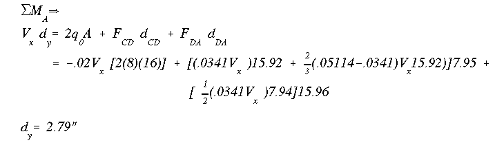
The shear center is located at (0", 0.6") from the centroid.
The resultant shear force will be equal to the vertical load at the tip. With no horizontal shear force and no product of inertia, the general shear flow equation reduces to
Again, assume q = 0 at a point (i.e., cut the section at corner 'A') and work around the cross section, finding the preliminary shear flow distribution.
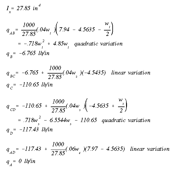
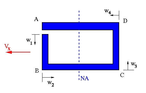
Each one of these equations should be checked for its maximum value location and whether there are any sign changes, indicating a change in the shear flow direction. To find a change in sign, set the equation to zero and solve for 'w'. If the result is within the limits of 'w' along that particular web, then there is a sign change. To find the location of the maximum value, take the derivative of the equation with respect to the 'w' and set the equation equal to zero. This part is just for quadratic or higher degree equations. The maximum for the linear equations will be at one end or the other. The analysis of one equation is shown here.
With this part done, the shear flow for the open section can be drawn as shown below.
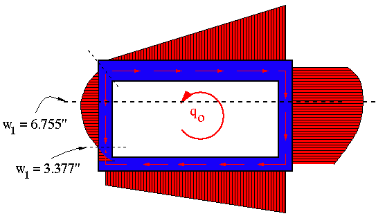
In the above diagram the values shown should be switched. The one at top is 3.377" and the one at the bottom is 6.755".
Sum the moments about corner 'A' to get the shear flow q0 needed to balance the moments. This time the forces along 'CD' and 'DA' are found by integration.

Add this constant shear flow to those found previously to get the final q distribution.
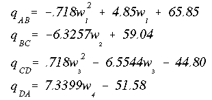
These equations should be analyzed again to determine any shear flow direction changes and locations of maximum shear flow. Two in particular are segments 'BC' and 'DA'. The location for the change in direction should be the same. Notice that in the above shear flow equations w2 and w4 are measured in opposite directions.
The final shear flow distribution is
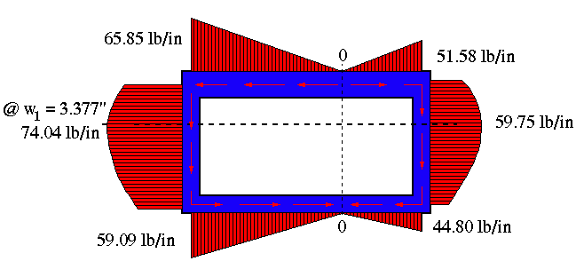
Notice that although the cross section is symmetric about the y axis, the shear flow distribution is not. This is because the vertical shear force is not on the axis of symmetry.
It is always a good idea to check equilibrium equations to make sure they are satisfied. In this case the summation of horizontal forces add up to zero as they should, and the summation of vertical forces add up to very close to 100 lb. The slight difference is due to the fact that the vertical component of the shear in the horizontal webs have been ignored. This idea was first discussed in the discussion of transverse shear loading of open sections in chapter III. Also if we were to take moments about any point, we will find the sum of moments due to shear forces balance the one due to external force.
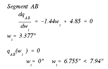
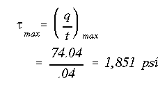
By examining the shear flow distribution and thickness variation, it is clear that the maximum shear stress is in segment 'AB' at w=3.377".
 To Section IV.1
 To Index Page of
Transverse Shear Loading of Closed Sections
To Index Page of
Transverse Shear Loading of Closed Sections