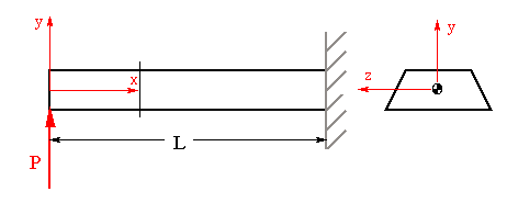
Consider a cantilever beam with a symmetric cross section subjected to a lateral (or transverse) force P at the tip. The shear and normal stresses induced by this force are required to be below the corresponding elastic limits of the material.
Next, we consider a transverse section located at some distance x from the free end of the beam as shown above. The bending moment at this section is related to the normal stress according to the equation

In order to go any further, we need to know how s x varies along the section. Recall from previous chapter that if the section is in the state of pure bending, then the normal strain vaires linearly. Furthermore, if the section is in elastic condition and the material is linearly elastic, then according to Hooke's law, normal stress would vary linearly as well. With that in mind, we need to determine whether the normal strain varies linearly in the presence of transverse shear force. Without getting too deep into the theory of elasticity, it suffices to say that if the beam is long compared to its cross section, then the normal strain does vary linearly. On the other hand, if the beam is short, then normal strain variation is in fact nonlinear when transverse shear force is present.
So we either have to limit our analysis to long beams or assume that the normal strain variation is linear regardless of the length of the beam. With the requirement of elastic condition and the use of linearly elastic materials, the general elastic bending formula described in the previous chapter can be used. In the presence of one moment component and zero product of inertia, the normal stress equation reduces to

The distance y is measured from the centroidal z axis (which in this case coincides with the neutral axis), Iz is the moment of inertia of the section about the z axis.
Relating the bending moment to the applied shear force P gives

The maximum normal stress, at section x, will occur at the farthest distance from the neutral axis. In this case the stress distribution indicates that distance to be to the top surface of the section as shown below.

To examine the shear force and associated shear stress created as a result of transverse force P, let's consider a beam segment highlighted in the figure below. While the left edge of the beam segment is free from any force in the x direction, the right edge is not due to the presence of sx. The question is how can equilibrium be maintained in this case? This points to the existance of a horizontal shear force H along the bottom surface (longitudinal surface) of the highlighted segment. The important point to notice first is that a transverse shear force results in the creation of a longitudinal shear force.

Now the equation for equilibrium of forces in the x direction is written as
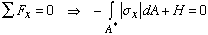
where A* represents the area of the beam section from y1 to c. Making appropriate substitutions and simplifying the resulting equation gives

The integral term represents a geometric quantity referred to as the moment of area,and is denoted by Qz. The subscript z indicates that the moment of area is obtained about the z axis. The equation for H can be written as

This equation indicates that the longitudinal shear force is an explicit function of x and an implicit function of y through the moment of area. At the tip section x is zero, hence H is zero for any value y. However, for any positive value of x, the variation in H depends on the location of y1. It can be shown that for y1 = 0, H reaches its maximum value whereas at y1 corresponding to the top and bottom surfaces, H goes to zero. Therefore, the longitudinal shear force H varies linearly with respect to x and quadratically with respect to y.
Now, divide both sides of the equation by x

Note that P times x represents the moment Mz at position x, and that in the limit as x approaches zero, Px/x simply represents the change in the bending moment which is simply equal to the transverse shear force at that location. Therefore, we can rewrite this equation as

The ratio of H over x represents the quantity known as the shear flow denoted by q. In this case, shear flow is acting along the longitudinal surface located at distance y1. For the problem described here, the shear flow can be written as

At a given position x, q varies according to the variation of Q. The equation for Q reveals that at the NA corresponding to y1 = 0, Q reaches its maximum value, and at y1 corresponding to the top and bottom surfaces, it will be zero.
To obtain the flexural shear stress along the longitudinal surface corresponding to y = y1, we simply divide q by the width of the longitudinal surface. If this dimension is denoted by t, then

The subscripts on t indicates that the longitudinal surface has a normal vector in the y direction and that the shear stress component is in the direction of x axis. Since shear stress in the longitudinal plane must be equal to that in the transverse plane, then the two subscripts can change places without any change in the right hand side of the equation. The equation above is known as the average flexural shear stress formula.
Although the value of shear flow is always maximum at the neutral axis location, we cannot conclude that shear stress will also be maximum there. The reason is that t may vary from one point to another, and that it is possible for a point other than the neutral axis to have the maximum shear stress. In order to calculate the maximum shear stress, the following relationship should always be followed.

Restrictions:
Before we can apply the average flexural shear stress formula, we must consider the restrictions that apply to this equation:
1. The section has to be homogeneous (made of a single material).
2. The section has to have an axis of symmetry, therefore, product of
inertia is zero.
3. The shear force V passes through the shear center of the section,
and is parallel to one of the two principal centroidal axes.
4. The shear stress at every point is below the corresponding elastic limit
of the material.
What if the longitudinal surface we considered in above derivation was not parallel to z axis? What would change in that case?
Answer:
To answer these questions, consider the figure shown below.
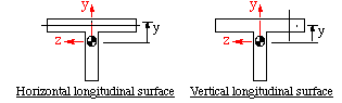
In the case of horizontal longitudinal surface, we will be calculating the yx or xy component of shear stress. To calculate Qz we use the area above the longitudinal surface. t in this case is equal to the distance from the left edge to the right edge of the top section. In the case of the vertical longitudinal surface, we will be calculating a different component of shear stress, i.e., tzx which is the same as txz on the transverse surface. In this case Qz can be found by considering the area to the right side of the longitudinal surface, and t would be equal to the flange thickness. This difference is demonstrated in the following discussion:
Shear Stress Components tyx and tzx
If V is along z direction, then the moment of inertia is that about the perpendicular axis or y axis in this case. For Vz loading, the flexural shear stress formula can be written as

Therefore, at a given point on the cross section we can calculate two components of shear stress depending on the orientation of the longitudinal surface. Generally speaking, one component is always much larger than the other thus, that would be the one of most interest in the analysis.
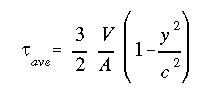
Table below gives equations for maximum shear stress for specific cross sections. The distance e is defined as the distance from the neutral axis to the point of maximum shear stress. The shear force V is normal to the NA and it acts along the vertical axis of symmetry, hence through the shear center. The maximum shear stress is given in terms of the ratio V/A.

Shear Stress Variation:
If we obtain the equation that describes the shear stress as a function of position on the cross section, it would be easy to find how shear stress varies from point to point as shown in the example figure below.
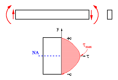
Knowing that the ratio V/I is constant for a given section, we need to only concentrate on the variation described by Q/t. For example, if we follow the derivation steps, we find the average flexural shear stress variation for a beam with rectangular cross section, as shown above, will be parabolic according to the equation
Shear Flow Variation:
The shear flow distribution at a given cross section is determined by writing the equation VQ/I, which is basically the shear stress multiplied by 't'. The shear flow distribution calculation can be seen in the example problems given at the bottom of this page.
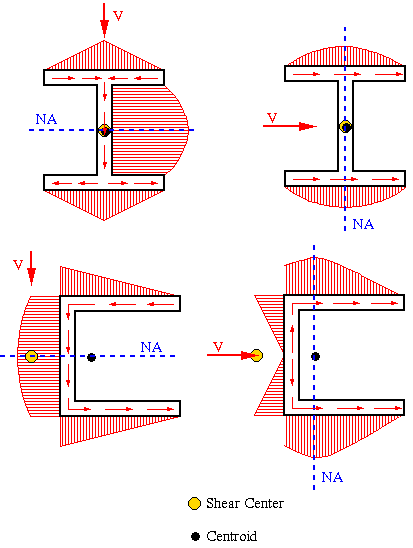
Here are some examples of shear flow diagrams for sections with at least one axis of symmetry. Each of these cases show the shear flow when the shearing load passes though the shear center.
In each of these shear flow diagrams, the maximum shear flow occurs at the neutral axis, which passes through the centroid of the section. This will also be the location of the maximum shear stress as the wall thickness is constant. Also notice how the shear load is perpendicular to the NA.
 To Section
III.4
To Section
III.4
 To Index Page of
Transverse Shear Loading of Open Sections
To Index Page of
Transverse Shear Loading of Open Sections
 To Section
III.2
To Section
III.2